What you will learn from this lesson
With Excel 97 you will:
-
Start a new workbook.
-
Enter and format a title.
-
Modify the text style and font
size.
-
Enter column headings and adjust
column width.
-
Move data.
-
Edit data.
-
Customize the enter key.
What you should do before you start this lesson
Creating a worksheet with Excel
97 is easy. To help you experience the power of Excel 97, you will use
excerpted material from Getting Americas Students Ready for the 21st
Century: Meeting the Technology Literacy Challenge, atechnology report
from the U.S. Department of Education.
Getting ready to create
a worksheet
-
Start Excel 97.
-
Open a new workbook.
Exploring the lesson
Excel 97 makes it easy to enhance
lessons and reports with data that you can enter and edit quickly. You
can create informational charts, grade books with calculating features,
data-based statistical programs, graphics, and simple task charts using
Excel 97.
Starting new workbooks
Excel 97 makes it easy to
design a new workbook to suit your purpose.
Creating a new worksheet
-
Open a new worksheet.
-
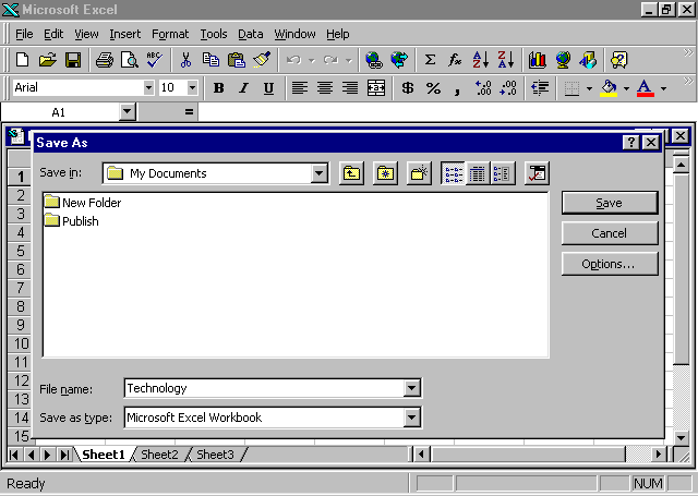
On the File menu, click
Save
As.
-
Type Assignment
2 as the file name.
-
Save to your h: drive

Entering and formatting titles
Using titles on the worksheets
makes it easier to read and understand the information shown. You can retain
the existing styles, create your own styles, or customize your own workbook
template. The next exercise illustrates how easy it is to enter and modify
font styles and sizes in your worksheet.
Entering and formatting
a title on the worksheet
-
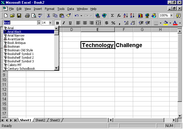
With Assignment 2
open, move the pointer to cell E3, type Technology Challenge, and
then press enter.
-
Click cell E3.
-
On the Formatting toolbar, click
the Font box, and click Arial. (You may have to use the down
arrow next to the Font box to find Arial.)
-
On the Formatting toolbar, click
the arrow next to the Font Size box, click 14, and then click
the Bold button.

Entering column headings and adjusting widths
Column headings help you and
others understand the data or information you have entered on your worksheet.
Sometimes the column heading is too large to fit into a column. Even though
it does not show the entire title or formula, the cell still contains everything
you entered into it. This exercise shows you how to increase or decrease
the column width to fit the information you are entering.
Entering column headings and
adjusting their widths
-
Using the Technology worksheet,
click cell B5, and type Dates in cell B5.
-
Press tab to go to cell C5,
and then type Elementary Schools.
-
Press tab to go to cell D5,
and then type Secondary Schools. One cell will overlap the other.
-
Press enter.
-
At the top of the worksheet,
position the pointer at the top of the grid between columns C and
D
until the pointer changes into a double-arrow line and then double-click.
-
Repeat step 5 between cells
D
and E.
-
Select the words Technology
Challenge, and move the + pointer to a cell line until it changes
to an arrow.
-
Click and drag the text to begin
in cell C3.
-
Save the worksheet (this is
still Assignment 2)
With these easy steps you can
customize a template or design your own workbook to present your information.
Arranging text with the Copy, Paste, and Cut commands
With Excel 97, it is easy to
modify data. When you use the features in Excel 97 to create a table, you
may decide on a different order of column heads or you may want to revise
them. It is important to make changes before you build a formula for the
chart in order to maintain correct calculations.
Using the Cut, Paste, and Copy
commands to arrange text
-
Open the Assignment
2 worksheet.
-
Double click cell C3, and click
Cut.
-
Double click cell C1, and click
Paste.
-
Double click cell D5, and click
Cut.
-
Double click cell D10, and click
Paste.
-
Double click cell C5, and click
Cut.
-
Double click cell D5, and click
Paste.
-
Double click cell D10, and click
Cut.
-
Double click Cell C5, and click
Paste.
-
Try dragging cell C5 andcell
D5 to new locations as you did in the previous exercise.
-
Close the file after saving
as Assignment 3.
Entering data
Using Excel 97 is a powerful
way to enter and display data or text. For example, you can have Excel
97 display a date showing the month, day, and year with the time, or showing
only the first letter of the month, followed by a two-digit year. Numbers
can be displayed as whole numbers, numbers with decimals, or numbers written
in scientific notation.
Entering data for growth
of World Wide Web sites in U.S. schools
-
Open the Assignment
2 workbook.
-
Starting in cell B6, type the
following information into the worksheet, under the corresponding headings.
-
Save your file as Assignment
4
|
Dates
|
Elementary
|
Secondary
|
|
1/1/95
|
85
|
110
|
|
4/1/95
|
160
|
360
|
|
7/1/95
|
225
|
380
|
|
10/1/95
|
250
|
660
|
|
1/1/96
|
425
|
900
|
|
4/1/96
|
800
|
1400
|
|
6/1/96
|
1100
|
1720
|
Doing simple calculations
Using Excel 97, you can perform
a wide range of mathematical calculations and functions according to what
you need from your data. To calculate sums (totals) and percentages, use
the mathematical operation of adding numbers to get a total, and then divide
each number that was just added by that total.
Calculating the sum of schools with Web sites
-
In the Assignment
4 workbook, click cell E5, type Total Sites,
and press enter.
-
Click cell E5 again, and on
the Formatting toolbar, click the Bold button.
-
Click cell E6, and on the Formula
toolbar click the Edit Formula button (the = sign).
-
Click the Functions arrow,
and choose Sum. (C6:D6 appears in the window.)
-
Click OK.
-
To sum each pair of numbers,
click E6, hold down, and drag the fill handle from E6 to E12.
Calculating the percentage of schools with Web sites by category
-
Click cell F5, type % of
Elem schools, and then press enter.
-
Click cell F5 again, and then
click the Bold button on the Formatting toolbar.
-
Click cell G5, type % of
Sec schools, and press enter.
-
Click cell G5 again, and on
the Formatting toolbar click the Bold button.
-
Click F6, and click the Edit
Formula button (the = sign).
-
Type C6/E6, and click
OK.
-
On the Formatting menu, click
Cells.
On the Number tab, choose Percentage, and then type 2
in the decimal places.
-
Click F6, and drag the fill
handle to F12 to calculate the percentage for each pair of numbers. Click
OK.
-
Repeat steps 3 through 8 for
Secondary Schools using the formula D6/E6 to calculate the percentage.
-
Save the worksheet as Assignment
4 and close it.
You should now have:
Assignment
1
Assignment
2
Assignment
3
Assignment
4
completed
Extensions
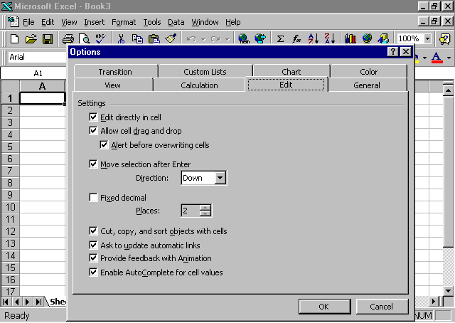
You can change the direction
in which the pointer moves when you press enter. If the default direction
is to the right, and you are entering data in a column, you can change
the default to down. You can change the direction of the pointer to support
your movements.
Customizing the enter key
Changing the direction
of the enter key
-
Open a new workbook.
-
On the Tools menu, click
Options.
-
Click the Edit tab.
-
Click Move selection after
Enter, and in the Direction box, click Right, and click
OK.
-
Repeat steps 1 through 4 to
change the direction back to Down.
-
Close the workbook without saving
it.

Summarizing what you learned
In this chapter you have explored
and practiced:
-
Starting and formatting a new
workbook.
-
Entering titles.
-
Modifying text style and font
size.
-
Entering column headings and
adjusting their widths.
-
Arranging text with the Copy,
Paste, and Cut commands.
-
Calculating simple formulas,
sums, and percentages.
-
Customizing the enter key.
|
